
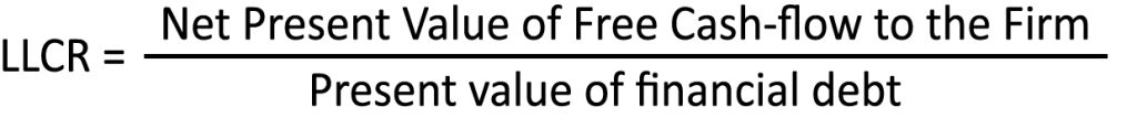
It is a solvency measure, calculated over the entire life period of financial debt. It is given by the present value of Cash-flow Available for Debt Service (CFADS), increased by the cash reserve (if present) available to repay the financial debt and divided by the amount of debt owed by the company at a given time elected for the evaluation. Only the cash-flows generated during the life period of the debt are to be considered, up to the expected cash earned in the last year of debt repayment.
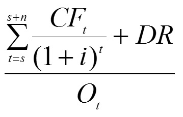
CFt = Cash-flow Available for Debt Service at year t
t = time variable
s = number of years expected to pay the debt back
i = WACC
DR = Cash reserve available to repay the debt (Debt reserve)
Ot = debt balance outstanding at time of evaluation
It is employed to assess the viability of a given amount of debt and consequently evaluate the risk profile and the related cost. It has a less immediate explanation compared to DSCR but when LLCR has a value greater than one this is usually a strong reassurance for investors.
The correct cash-flow to be used to calculate LLCR is not the Operating Cash-flow (also called Unlevered) but the Cash-flow Available for Debt Service (CFADS).
Such a quantity is the total amount of resources available to the company in order to pay back debt principal and to cover the related financial charges.
Cash-flow Available for Debt Service
The first step is to calculate Cash-flow Available for Debt Service, which represents the free amount of money the company can employ to pay back its debt bank.
This is none other than the Unlevered Operating Cash-flow plus specific components of income that may not be related to the company’s operating activity (e.g. non-operating income and expenses, financial charges, etc.)
However, for the sake of completeness, two different schools of thought can be found as to the matter of the calculation of this cash-flow.
Operating Profit (EBIT)
– Profit Tax
+ Depreciation and amortization
+ Adjustments for non-cash items
+/- Adjustments for changes in working capital
+/- Capex
CFADS
+ Proceeds from borrowings
– Repayment of borrowings
– Interest expense
+/- Adjustments for financial activities
+ Interest income
+/- Equity
Free Cash-flow to Equity
– Shares Paid
Net Cash-flow
Operating Profit (EBIT)
– Profit Tax
+ Depreciation and amortization
+ Adjustments for non-cash items
+/- Adjustments for changes in working capital
+/- Capex
Operating Cash-flow
+/- Adjustments for financial activities
– Interest Income
+/- Equity
Cash-flow available for debt service
+ Proceeds from borrowings
– Repayment of borrowings
– Interest expense
Free Cash-flow to Equity
– Shares Paid
Net Cash-flow
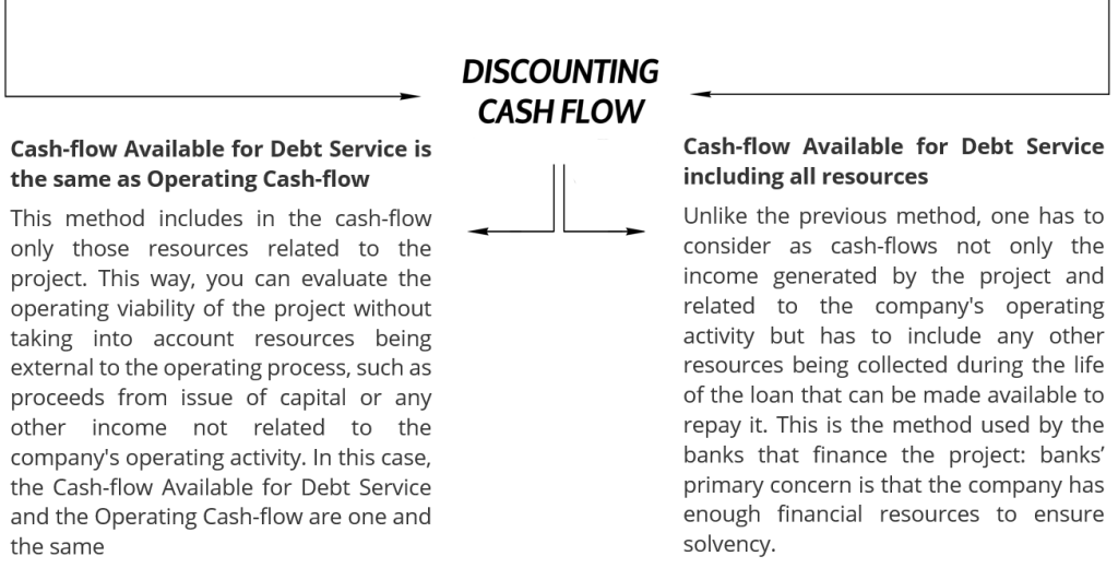
We prefer option number two, the one including non-operating income in the cash-flow for debt service.
LLCR calculation: an example
Let’s consider the scenario described by the following cash-flow statement:
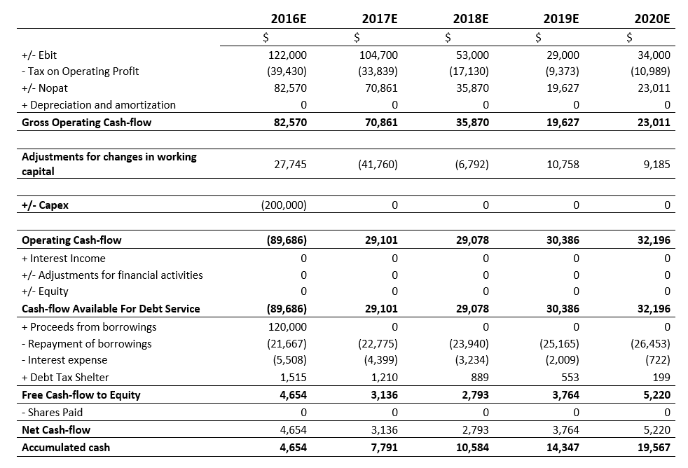
In 2016, the bank grants the company $ 120,000 on a loan, the amount is used to partially cover an investment of $ 200,000.
The loan repayment plan stipulates a five-year duration, involving monthly installments at an annual interest rate of 5%, The initial installment is due on January 31, 2016, The last year expected for repayment is 2020. The remainder of the investment is covered by the expected cash-flow generated by the company, since the plan does not envision a capital issue.
We use a reporting model that starts from EBIT and makes a series of adjustments to account for non-monetary values. We also calculate NOPAT by providing for Taxes on Operating Profit (see Article) to take account of the deductibility of financial charges.
As can be seen from the example, in the first year (2016) both the Operating Cash-flow and the Cash-flow for the Debt Service are negative because of the investment made.
However, this cash requirement is covered by the funds obtained from the bank loan of $ 120,000, which also covers the repayment of the first installment. In fact it’s all but unusual during the start-up phase that the company requires a slightly higher amount of funding to cover the first installment as well, since it is difficult for the company to be fully profitable in the first year.
In the forecast years 2017-2020 both the Operating Cash-flow and the Cash-flow For the Debt Service are positive and the company is then able to repay the loan installments.
Let’s now calculate LLCR using the formula we have previously reported, assuming a 5% discount rate (WACC):
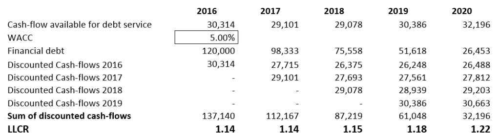
LLCR assesses the debt viability for each projected year so to associate to each stage of the financial plan a figure that measures its degree of “coverage”, that is stability of the project should any variations occur in the expected scenario (e.g. lower sales than expected or unexpected extraordinary costs).
To calculate LLCR of year 2016 (evaluated at 31/12/2016), it is necessary to discount all expected cash flows at that date, beginning with the cash-flow projected for 2016 and until the last year when debt is expected to be repaid, taking into account the whole “life” of the loan.
We obtain the quantity mentioned in the previous table as Sum of discounted cash-flows (equal to $ 137,140 in 2016).
The discount factor, that being the quantity each expected cash-flow has to be multiplied by to obtain the present value at 31/12/2016, depends on the discount rate (WACC) and on the number of years between the time of the evaluation and the time when each-cash flow is expected to be generated. For example, in order to calculate the present value at 31/12/2016 of the cash-flow expected for year 2020, the latter has to be multiplied by a factor equal to:
(1+WACC)-3 = (1 + 0,05)-3 = 0,86
Sum of discounted cash-flows (2016) = FC2016 + FC2017 x (1 + WACC)-1 + FC2018 x (1 + WACC)-2 + FC2019 x (1 + WACC)-2 + FC2020 x (1 + WACC)-4 = € 30.314 + € 27.715 + € 26.375 + € 26.248 + € 26.488 = $ 137.140
Note that the cash-flow of year 2016 does not have to be multiplied by any discount factor because it is obtained at the very time of the evaluation, i.e. 31/12/2016.
Once expected cash-flows have been discounted, their sum has to be simply divided by the value of the debt that these amounts have to repay, in the example being equal to $ 120,000. This will yield to the value of LLCR for year 2016 (1.14). As this value is greater than one, one can conclude that, as of 31/12/2016, debt is sustainable, with a certain margin, as the company is expected to generate higher resources (as a present value) compared to the value of the debt it is committed to repay.
It is also worth noting that Cash-flows For Debt Service must also include the proceeds from the financing activity itself, i.e. the capital borrowed from the lenders. In fact, there is no compelling reason to exclude such resources from the assessment of the financial viability, since debt capital is in itself an essential component to ensure the sustainability of the project and once that is obtained, it represents resources available (as a whole or in part) for the repayment of the debt itself.
This also explains why the Operating Cash-flow and the cash-flow from extraordinary activity (negative and equal to $ 89,686) must be summed up with the $ 120,000 amount obtained through the loan, so to have the actual Cash-flow For Debt Service, equal to $ 30,314.
Concerning the value of the debt to be considered to calculate LLCR, this must be equal to the debt balance that is due at the beginning of the year of evaluation, in the example on 01/01/2016. Bear in mind that each of the Cash-flows For Debt Service is calculated excluding the repayment of the debt and therefore must be compared with the value of the debt outstanding before the payment of the principal. In other words, if we consider cash-flows before debt repayment, the value of the debt must be accordingly considered. However, the formula commonly used in literature takes account of time t, but probably this is the result of a misunderstanding because in these sources a school hypothesis is usually described where in the first year (2016 in our example) no debt repayment is expected.
We can safely say that in the many plans we have analyzed, this error is always there in the formula. This clearly implies greater sustainability and bankability of the plan because it yields to a higher LLCR.
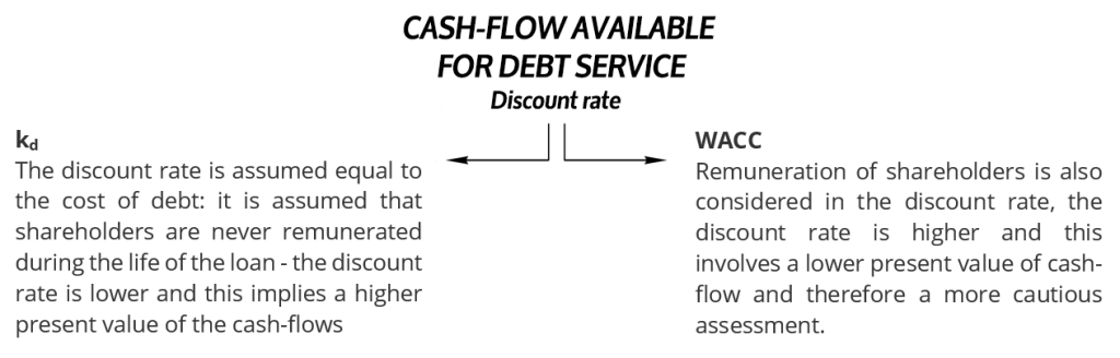
The discount rate
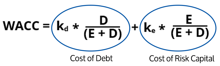
In our example, we used WACC as a discount rate to obtain the cash-flows present values. WACC is a rate that remunerates all the resourced, both as debt and as risk capital, used by the company to finance its business. Some authors, however, use the cost of debt as a discount rate without taking into account the remuneration of the shareholders.
Are they correct? It depends on how we calculate the Cash-flow For Debt Service and if we expect the remuneration of the shareholders as well.
If we discount Cash-flows For Debt Service at the sole cost of debt we are assuming that during the loan life and until it is completely repaid, no reward is paid to shareholders even if they have invested resources in the project. In this case, the discount rate would be lower (in fact, the second part of the WACC formula would be omitted) resulting in a higher value of discounted amounts and consequently higher debt sustainability. When the plan is submitted to a bank, not including a shareholder remuneration may seem unlikely and in any case the use of WACC as a discount rate guarantees a degree of caution in the assessment of the project. When LLCR is calculated using WACC as a discount rate it responds to the need to verify that even if a certain remuneration is required by shareholders the bankability and debt sustainability is still assured.
Conclusions:
The importance of taxes for WACC
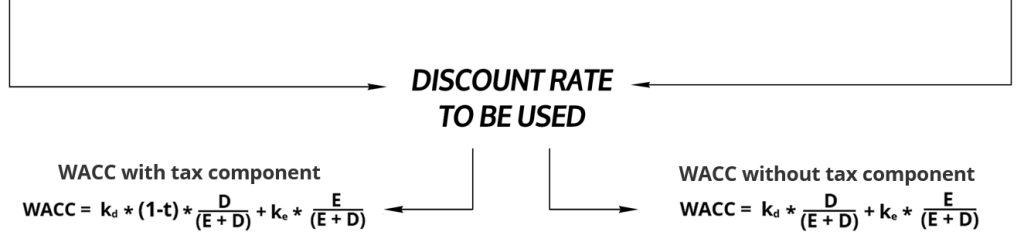
An important point to keep in mind is that in the WACC formula you have to consider the multiplier (1-t) only if the discounted cash-flow is calculated taking into account the deductible portion of the financial charges, which in turn implies an higher tax value. We have already discussed the issue in a previous article you can refer to for all details. For this reason, the correct WACC formula is the one above.
Depending on the model of cash-flow statement used (taking into account Taxes on Operating Profit or not) you have to consider the term (1-t) in the WACC formula, or not.
Cash-flow with Tax on Operating Profit
Operating Profit (EBIT)
-Tax on Operating Profit
= NOPAT
+ Depreciation and amortization
+ Adjustments for non-cash items
+/- Adjustments for changes in working capital
+/- Capex
+ Interest Income
+/- Adjustments for financial activities
+/- Equity
= Cash-flow available for debt service
Cash-flow without Tax on Operating Profit
Operating Profit (EBIT)
– Profit Tax
+ Depreciation and amortization
+ Adjustments for non-cash items
+/- Adjustments for changes in working capital
+/- Capex
+ Interest Income
+/- Adjustments for financial activities
+/- Equity
= Cash-flow available for debt service